
Networks are omnipresent, but not all networks are easily conceptualized in the physical world. Some networks, like our nervous system of interconnected neurons, railway lines, and electrical power grids, are physical objects embedded in 2-dimensional or 3-dimensional physical space, where the nodes represent points in space. On the other hand, networks such as economic networks and social networks are abstract objects representing interactions between entities. For some of these networks, a physical intuition is still possible. For instance, nodes may contain a list of features, and edges are drawn based on the relationship between these features. However, the dimension of this space (number of features) can be large, making interpretability difficult. In general, the majority of networks, like the World Wide Web or biochemical networks inside living cells, come with no intrinsic notion of space. Nodes have no spatial coordinates or features to facilitate physical intuition; the network represents only the abstraction of a set of entities with some connections between them.
 Networks with edges coloured by their dynamic Ollivier-Ricci curvature at two different resolutions. Nodes represent clusters based on maximising the average edge curvature within a cluster.
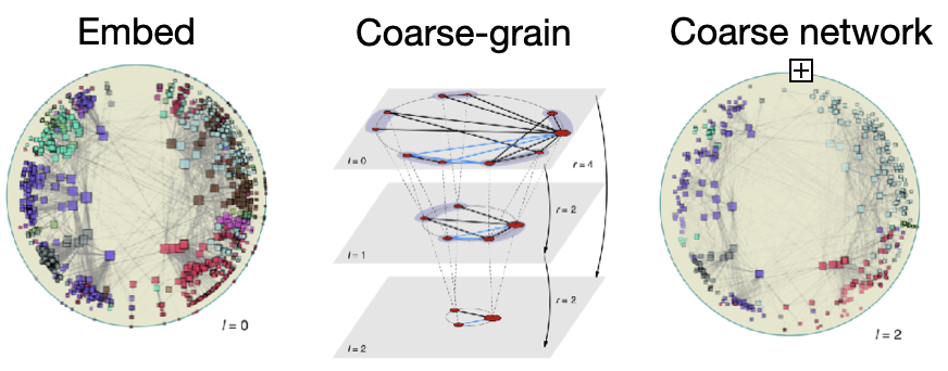
Having a space in which the network can be laid out, a so-called embedding space turns out to be very useful for analyzing networks. For example, assuming that the network’s nodes follow a continuous structure (manifold approximation), connections respecting this continuity can be preserved while those violating it may be ignored. This assumption allows unfolding the network in a 2D embedding space, often very useful to reveal its structure. Another example relates to complex networks, which obey power-law degree distributions. García-Pérez and colleagues found that nodes in complex networks can be naturally embedded in hyperbolic space, known from M.C. Escher drawings. Remarkably, when nodes are clustered based on proximity in hyperbolic space, the community structure is preserved—meaning the network structure is invariant under hyperbolic geometry. Without an embedding space, there is no inherent notion of direction in a network, making it harder to understand the spreading of information. Finding an embedding space may also be used to study the spreading of dynamical processes in networks, such as epidemics. Helbing and colleagues studied the spreading of infectious diseases on networks by defining an effective distance that maps nodes into a space where the wavefront started at a given node reaches points at the same time at a given radial distance. Using this distance to map the network into 2D space revealed node communities in which the infection started at a given point in the network arrives at the same time. Such information is useful for controlling the infectious process by blocking targeted edges.
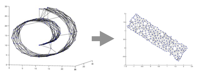 Manifold approximation (Tennenbaum et al., 2000)
 Hyperbolic space embedding (Garcia-Perez et al., 2018)
 Dynamic embedding (Helbing et al., 2013)
While embeddings are useful, they also have their dangers. In fact, for many networks, embedding their nodes into any normed vector space will necessarily lose much of the information encoded in the connectivity. The process of embedding stretches and shrinks the edges between pairs of edges by amounts comparable to the length of the edge itself. Many techniques in the field of non-linear dimensionality reduction deal with cleverly ‘distributing’ these distortions to preserve relevant features of the data while losing others. For example, the t-SNE method aims at preserving the distance between nearby points while allowing points far away to be embedded arbitrarily. However, it is currently not well understood what features of the network one should preserve to create meaningful embeddings.
An alternative to using embeddings could be to define the geometry of the network based on analogues borrowed from differential geometry, which deals with the geometry of continuous spaces. One way to define geometry in continuous spaces is through the concept of curvature. Consider two points x and y (on a manifold) and move them in parallel in an arbitrary direction to points x’ and y’. Depending on the geometry of the space, the transported points will be closer or further away. By computing the average distance of points nearby x and points nearby y relative to the distance of x and y, one can define the Ricci curvature in direction xy.
 Consider two points *x, y in a space. Then move x a small distance in a direction given by the white arrow. Likewise, move y in the same direction (known as parallel transport). Depending on the curvature of the space, the transported points are on average closer or further.*
Generalizing the notion of Ricci curvature to networks is less than straightforward. Because curvature requires a notion of direction, which is lacking in networks, there is no unique way to define network geometry. It is therefore not clear which one will yield insights into the structure of the network. In this work, we studied the notion developed by Ollivier, which, ‘simply’ put, replaces the average distance between points x’ and y’ with the optimal transport distance. The optimal transport or Wasserstein distance represents the least energy required to move a pile of sand to a pit. The distribution on the neighbors x’ can also be thought of as units of sand (to be transported), while the distribution on the neighbors y’ as unit holes (to be filled in). Intuitively, when x and y share neighbors, the holes are already filled in without moving mass. Thus, the higher the number of shared neighbors, the lower the transportation distance and the higher the curvature.
 The Ollivier-Ricci curvature is defined by generalizing the Ricci curvature by replacing the average distance of points *x’ and y’ by the optimal transport distance.*
When one computes the Ollivier-Ricci curvature only between adjacent nodes on the network (endpoints of an edge), it turns out to be remarkably intuitive. There is a deep analogy between the curvature of canonical networks and canonical geometric spaces, as illustrated by the figure below.
 Correspondence between the Ollivier-Ricci curvature (top) and Ricci curvature (bottom) on canonical geometries.
Our idea was to replace the notion of the neighborhood of points x, y by diffusion processes started at points x, y. The diffusion processes distribute mass unevenly and on all nodes, rather than just the neighbors, which makes the problem more interesting. In the following figure, the red lines show the edge connecting two points, and the orange and blue semi-circles show the evolving diffusions. One can see that the diffusions stay trapped in well-connected regions of the network for some time before spreading to the rest of the network. In Ollivier’s definition, the distance between neighboring points is equally weighted because all neighbors carry the same mass. By considering diffusions, we place different importance on different pairs of points, i.e., different amounts of mass are placed over nodes as given by the size of semi-circles. Moreover, as the diffusions propagate, the dynamic geometry captures increasingly coarser features of the network. Therefore, instead of a single geometric object (like in classical Ollivier-Ricci curvature), we obtain a family of geometric objects parametrized by the time of diffusion.
 Propagation of a pair of diffusions started at adjacent nodes in different clusters
 Propagation of a pair of diffusions started at adjacent nodes in the same clusters
Because of the different timescales on which pairs of diffusions spread in the network, one may wonder how this could be reflected in the curvature of the network. One way to answer this is to visualize the curvature evolution, i.e., plotting the curvature value of each edge ij at a given point in time τ that marks the state of the diffusions. An observation is that the curvature distribution splits up into ‘bundles’ as time progresses. This observation makes sense by looking at the small networks in the insets. When both diffusions start within clusters (well-connected network regions), they become quickly overlapping, thus increasing the curvature. Meanwhile, for other edges spanning different clusters, the diffusions tend to overlap less and thus the curvature increases more slowly. One can now realize that, eventually, the diffusions started from anywhere will fully overlap, which will cause the curvatures to increase to the value of one as time goes to infinity. However, interesting structures are found at smaller times when the network diffusions are still far from being fully dispersed.
In our work, we found that the differences in the curvatures of bundles can be related to the rate of information exchange between diffusions. This is mathematically characterized by the rate of mixing of diffusions. More precisely, when the curvature reaches 0.75, as shown by the red dashed line, the corresponding pair of diffusions have mixed well. Note, they have not fully dispersed yet (they are not at stationarity). Instead, from this point in time onwards, they will move together until the dispersed state. Looking at the points in time where some diffusion pairs have mixed, shown by the vertical dashes, one can find edges that have still a long way until mixing. We call these curvature gaps that indicate bottlenecks in information flow. These bottlenecks can be visualized too! In the middle figure, we see that the curvature is lower between clusters than within clusters. In the right picture, the curvature is similar for edges within clusters and across the top and bottom clusters, while lower for those between the left and right clusters. These patterns reflect different scales in the graph revealed completely geometrically!
 Curvature distribution at different times of the diffusion processes. Initially, all curvatures are 0. As time progresses, the distribution separates into ‘bundles’ and develops gaps. When the curvature reaches 0.75, the diffusions are well-mixed between regions spanned by the given edge. Looking at the curvature distribution at timepoints where the individual bundles reach 0.75 visually reveals multiple clusters based on the sign of the curvature.
To take this idea further, we looked for ways to modify the information flow between clusters. We accomplished this in two ways. First, we changed the ratio between the number of edges between clusters to that within clusters, called the edge density ratio r. A low edge density ratio means that it is hard for the diffusions to pass from one cluster to another, essentially creating more contrast between the communities. Second, but more subtle, we reduced the number of edges in the graph while maintaining the edge density ratio. This has the effect of reducing the mean degree k, the average number of edges connected to each node. The figure below illustrates on a graph with two clusters that as we remove more edges the communities become less distinguishable.
 (right) As the network becomes sparser, there is less information about the community structure. (left) Initially, the node degrees are evenly distributed around a mean (~60), which becomes disordered with many low degree and a few high degree nodes.
We then simulated many such graphs for different mean degrees (k) and edge density ratios and computed the curvature gap. From the following figure, it is clear that when the mean degree is lower, a lower edge density ratio suffices to establish a curvature gap. This observation makes sense: the fewer edges the graph has, the larger the contrast needs to be to find communities reliably. As the edge density ratio increases, the curvature gap is no longer different from background noise, shown by the black horizontal line. What is more surprising is that the point at which the curvature gap disappears for a given average degree is the final point when the edges can convey any information about the community structure. In fact, beyond this point, known as the Kesten-Stigum bound, there is no efficient algorithm that can tell the communities apart. When we look at the distribution of the transition points for different mean degrees, the prediction of the curvature gap lies very close to the theoretical prediction! In the paper, we show that this is no coincidence; in
Because of the strong link between curvature gap and network communities, one natural application of our theory is network clustering or community detection. The nodes of a network can be grouped into communities based on different criteria, so the ‘correctness’ of communities is in general a subjective matter. However, clustering networks based on finding curvature gaps, i.e., directions of limited information flow is a valuable viewpoint. Firstly, because the curvature distribution encodes all information about the communities (disclaimer: our results show this for stochastic block model graphs), clustering using curvature performs substantially better than classical node-clustering methods such as spectral clustering. Secondly, because of the association of low curvature edges with bottlenecks, communities are interpreted as containing nodes that share redundant information and that easily disconnect from the rest of the network. In other words, breaking low curvature edges is expected to have the largest effect on the information spreading.
To show that our framework can truly find useful applications, we clustered two real-world networks: the European power grid network and a network of C. elegans neurons constructed based on the similarity of their homeobox gene expressions (homeobox genes are genes expressing proteins called transcription factors). Sparing the details for the interested reader, we could reveal striking information in both networks. Clustering the European power grid revealed clusters representing countries and other geographical regions on one scale as well as clusters representing the historical split between Eastern and Western Europe on another scale. All this information from nothing more than the wiring of electrical power lines! Not less interesting is the C. elegans gene expression network. Clustering this network revealed the anatomical type of most of the 302 neurons in the worm! In the future, we hope to find more links between the communities identified from the curvature distribution to physical or biological properties of real-world networks.
 European power grid network and C. elegans neurons clustering
 C. elegans neurons clustering
 C. elegans neurons clustering
Gosztolai, A., Arnaudon, A. Unfolding the multiscale structure of networks with dynamical Ollivier-Ricci curvature. Nature Communications 12, 4561 (2021) code